Base User guide

# Author: Iulii Vasilev <iuliivasilev@gmail.com>
#
# License: BSD 3 clause

First, we will import modules and load data

import survivors.datasets as ds
import survivors.constants as cnt

X, y, features, categ, sch_nan = ds.load_pbc_dataset()
bins = cnt.get_bins(time=y[cnt.TIME_NAME], cens=y[cnt.CENS_NAME])
print(bins)

[  41   42   43 ... 4189 4190 4191]

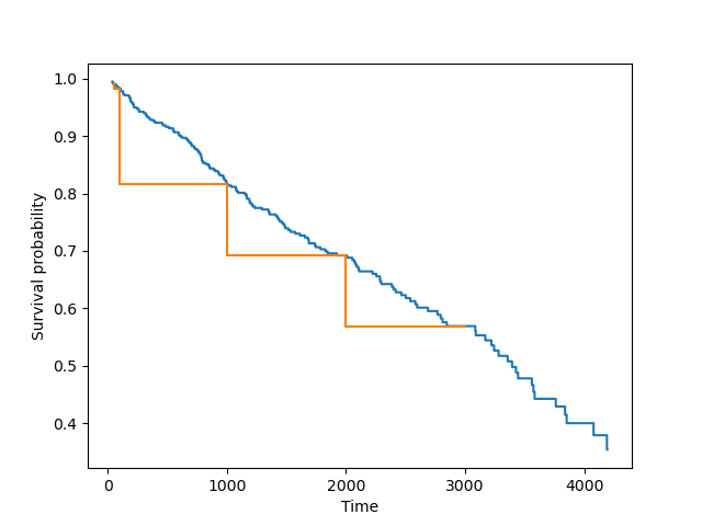
Build Nonparametric KaplanMeier model and visualize survival function

import survivors.visualize as vis
from survivors.external import KaplanMeier

km = KaplanMeier()
km.fit(durations=y["time"], right_censor=y["cens"])
sf_km = km.survival_function_at_times(times=bins)
vis.plot_survival_function(sf_km, bins)

bins_short = [50, 100, 1000, 2000, 3000]
sf_km_short = km.survival_function_at_times(times=bins_short)
vis.plot_survival_function(sf_km_short, bins_short)

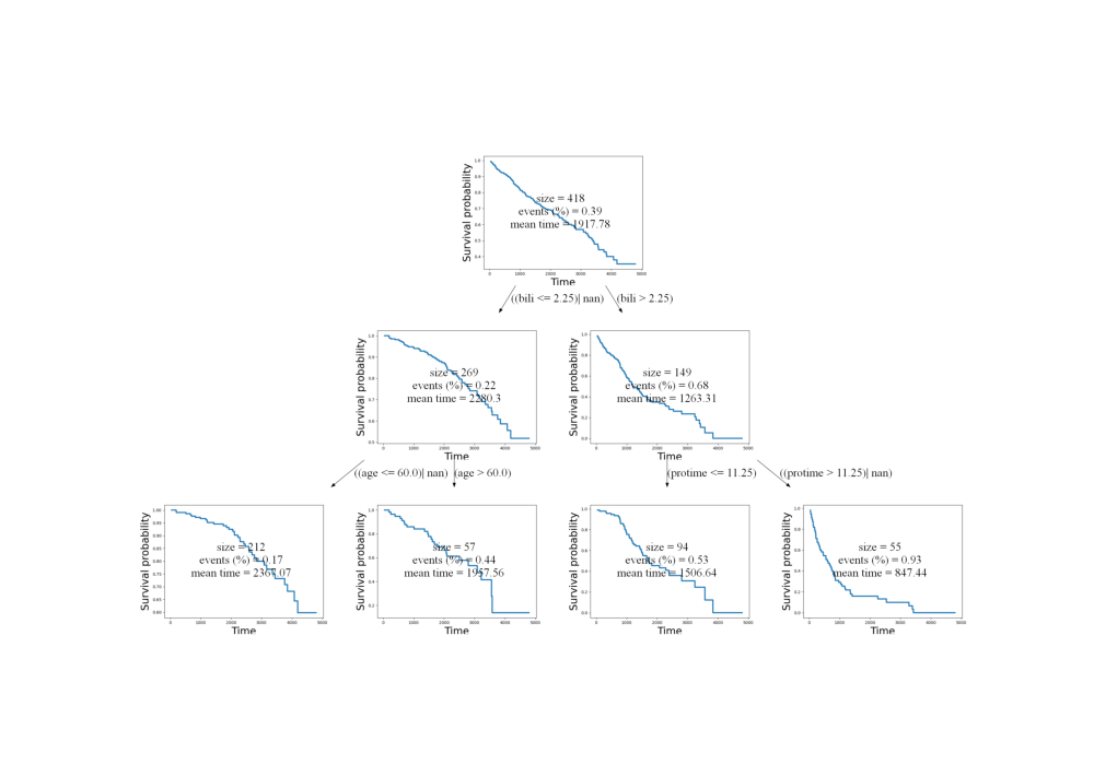
Build Tree

from survivors.tree import CRAID

cr = CRAID(criterion='logrank', depth=2, min_samples_leaf=0.1, signif=0.05,
           categ=categ, leaf_model="base")
cr.fit(X, y)

sf_cr = cr.predict_at_times(X, bins=bins, mode="surv")
chf_cr = cr.predict_at_times(X, bins=bins, mode="hazard")

print(chf_cr.shape)

(418, 4151)

Plot dependencies

import matplotlib.pyplot as plt
cr.visualize(target=cnt.TIME_NAME, mode="surv")

image = plt.imread(f'{cr.name}.png')
fig, ax = plt.subplots(figsize=(10, 7))
ax.imshow(image)
ax.axis('off')
plt.show()

Individual prediction

print("Target:", y[0])
print(cr.predict(X, target=cnt.TIME_NAME)[0])
print(cr.predict(X, target=cnt.CENS_NAME)[0])
print(cr.predict(X, target="depth")[0])

Target: (True, 400.)
847.4363636363636
0.9272727272727272
2.0

Building ensembles of survival trees

from survivors.ensemble import BootstrapCRAID

bstr = BootstrapCRAID(n_estimators=10, size_sample=0.7, ens_metric_name='IBS_REMAIN',
                      max_features=0.3, criterion='peto', depth=10,
                      min_samples_leaf=0.01, categ=categ, leaf_model="base")
bstr.fit(X, y)

sf_bstr = bstr.predict_at_times(X, bins=bins, mode="surv")

fitted: 10 models.

Evaluation of models

import survivors.metrics as metr

mean_ibs = metr.ibs(y, y, sf_bstr, bins, axis=-1)
mean_ibs  # 0.071
ibs_by_obs = metr.ibs(y, y, sf_bstr, bins, axis=0)
ibs_by_obs  # [0.0138, 0.038, ..., 0.0000, 0.0007]
ibs_by_time = metr.ibs(y, y, sf_bstr, bins, axis=1)
ibs_by_time  # [0.0047, 0.0037, ..., 0.0983, 0.3533]

print(ibs_by_time.shape)

(4151,)

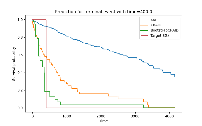
Predict comparison

vis.plot_func_comparison(y[0],
                         [sf_km, sf_cr[0], sf_bstr[0]],
                         ["KM", "CRAID", "BootstrapCRAID"])

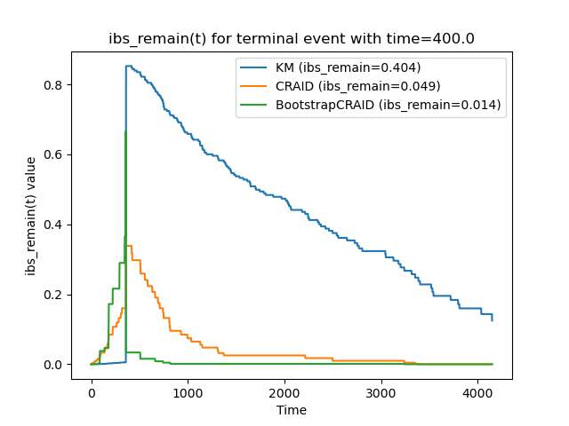
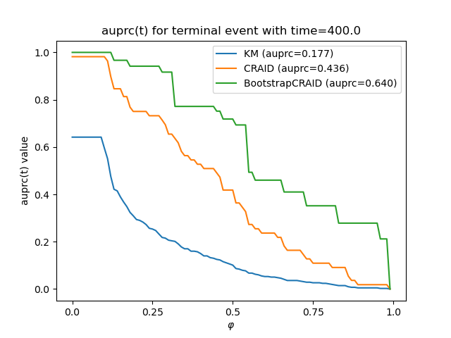
Quality comparison in time

vis.plot_metric_comparison(y[0], [sf_km, sf_cr[0], sf_bstr[0]],
                           ["KM", "CRAID", "BootstrapCRAID"], bins, metr.ibs_remain)
vis.plot_metric_comparison(y[0], [sf_km, sf_cr[0], sf_bstr[0]],
                           ["KM", "CRAID", "BootstrapCRAID"], bins, metr.auprc)

• 
•